Grid to a map

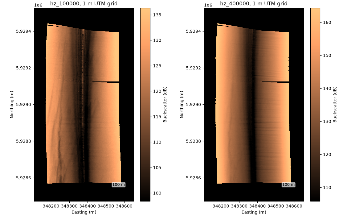
Once every sample has a latitude and longitude (the georef step), grid_channel() resamples a channel onto a regular UTM grid and to_geotiff() writes it for a GIS.

The line is from a Benthos SIS-1624 survey in the Irish Sea (XTF written by Isis), which records altitude and navigation, so the standard corrections are enough. The GeoTIFF needs the geo extra (rioxarray).

Data: JNCC mid-Irish Sea, Open Government Licence v3.0 (see Example data).

Usage: python examples/gallery/plot_grid_to_a_map.py [output_dir]

# 2026 rshomberg@uri.edu

import sys
from pathlib import Path

import matplotlib.pyplot as plt
import numpy as np
from matplotlib.patches import Rectangle
from matplotlib.ticker import FuncFormatter

from sidescanpy import datasets
from sidescanpy.grids import grid_channel, to_geotiff
from sidescanpy.io import read_and_convert
from sidescanpy.log import configure_logging
from sidescanpy.processing import (
    apply_tvg,
    compute_geometric_ranges,
    compute_georeferencing,
    interpolate_aux_onto_pings,
    slice_by_range,
)
from sidescanpy.viz import plot_grid_coverage, plot_gridded_raster

out = Path(sys.argv[1]) if len(sys.argv) > 1 else Path(".")
out.mkdir(parents=True, exist_ok=True)
configure_logging("INFO")

Navigation in this file is sample-and-hold: each position repeats for several pings until the next fix arrives. interpolate_aux_onto_pings() interpolates between the real fixes, not the repeated entries, which puts the pings about 0.65 m apart.

survey = read_and_convert([datasets.fetch("jncc_mid_irish_sea_MIS11_0.xtf")], fmt="xtf")
survey = interpolate_aux_onto_pings(survey)
survey = apply_tvg(survey)
survey = compute_geometric_ranges(survey)
survey = compute_georeferencing(survey)

Grid each frequency at 1 m, leaving out the water column. Heading jitter and a few longer jumps between fixes leave empty cells; inverse-distance weighting with a 4 m search radius fills them from the nearest samples. North is up; the dark stripe is the nadir under the towfish.

fig, axes = plt.subplots(1, 2, figsize=(11, 7), constrained_layout=True)
for ax, freq_key in zip(axes, ["hz_100000", "hz_400000"]):
    ds = slice_by_range(survey.get_frequency(freq_key).dataset, min_m=5)
    raster = grid_channel(ds, resolution_m=1.0, method="idw", max_search_radius_m=4.0)
    to_geotiff(raster, out / f"mid_irish_sea_{freq_key}.tif")
    plot_gridded_raster(raster, fig=fig, ax=ax, cmap="copper", vmin_pct=2, vmax_pct=98,
                        title=f"{freq_key}, 1 m UTM grid")
fig.savefig(out / "grid_to_a_map.png", dpi=110)

Choosing how cells are filled

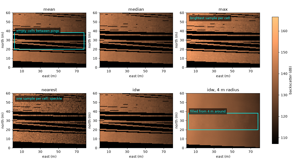
Each cell takes the samples within the search radius of its centre (by default 1.5 cells) and combines them with one of the ResamplingMethod values. Here 100 pings of the 400 kHz channel are gridded at 0.5 m with each, plus inverse-distance weighting with the 4 m radius used above, all on one color scale and shown over the same 80 m by 60 m window. The pings are about 0.65 m apart on average, but this file’s positions bunch up and jump between fixes (by up to 5.7 m between pings 405 and 409, inside the box), so at 0.5 m the default radius leaves stripes of empty cells between pings; the 4 m radius fills them.

ds400 = slice_by_range(survey.get_frequency("hz_400000").dataset, min_m=5)
lines = ds400.isel(ping=slice(360, 460))
choices = [("mean", None), ("median", None), ("max", None), ("nearest", None), ("idw", None), ("idw", 4.0)]
rasters = {}
for method, radius in choices:
    label = method if radius is None else f"{method}, {radius:g} m radius"
    rasters[label] = r = grid_channel(lines, resolution_m=0.5, method=method, max_search_radius_m=radius)
    print(f"{label:22s} cells with data {r.data_coverage:5.1%}, median {np.nanmedian(r.backscatter):6.1f} dB")

pooled = np.concatenate([r.backscatter[np.isfinite(r.backscatter)] for r in rasters.values()])
lo, hi = np.percentile(pooled, [2, 98])
x0, y0 = 348250.0, 5929100.0  # south-west corner of the window (UTM 30N)
fig, axes = plt.subplots(2, 3, figsize=(12, 6.6), constrained_layout=True)
for ax, (label, r) in zip(axes.flat, rasters.items()):
    plot_gridded_raster(r, fig=fig, ax=ax, cmap="copper", vmin=lo, vmax=hi, show_colorbar=False,
                        show_scale_bar=False, title=label)
    ax.set(xlim=(x0, x0 + 80), ylim=(y0, y0 + 60), xlabel="east (m)", ylabel="north (m)")
    ax.xaxis.set_major_formatter(FuncFormatter(lambda v, _: f"{v - x0:.0f}"))
    ax.yaxis.set_major_formatter(FuncFormatter(lambda v, _: f"{v - y0:.0f}"))
gap = dict(fill=False, ec="cyan", lw=1.5)
label_box = dict(fc="black", alpha=0.6, lw=0)
axes[0, 0].add_patch(Rectangle((x0 + 2, y0 + 20), 76, 18, **gap))
axes[0, 0].text(x0 + 4, y0 + 39, "empty cells between pings", color="cyan", fontsize=9, bbox=label_box)
axes[0, 2].text(x0 + 4, y0 + 53, "brightest sample per cell", color="cyan", fontsize=9, bbox=label_box)
axes[1, 0].text(x0 + 4, y0 + 53, "one sample per cell: speckle", color="cyan", fontsize=9, bbox=label_box)
axes[1, 2].add_patch(Rectangle((x0 + 2, y0 + 20), 76, 18, **gap))
axes[1, 2].text(x0 + 4, y0 + 39, "filled from 4 m around", color="cyan", fontsize=9, bbox=label_box)
fig.colorbar(axes[0, 0].collections[-1], ax=axes, shrink=0.8, label="backscatter (dB)")
fig.savefig(out / "grid_methods.png", dpi=150)

mean                   cells with data 34.6%, median  137.7 dB
median                 cells with data 34.6%, median  138.0 dB
max                    cells with data 34.6%, median  145.6 dB
nearest                cells with data 34.6%, median  137.8 dB
idw                    cells with data 34.6%, median  137.7 dB
idw, 4 m radius        cells with data 53.9%, median  138.3 dB

mean, median and idw agree to within a few tenths of a dB. max takes the brightest sample in each cell and so sits about 8 dB higher, and nearest keeps the speckle of single samples. The mean is the default; idw with a search radius of a few ping spacings is the usual choice for a map with no holes, at the cost of smoothing detail smaller than that radius.

How many samples fell in each cell

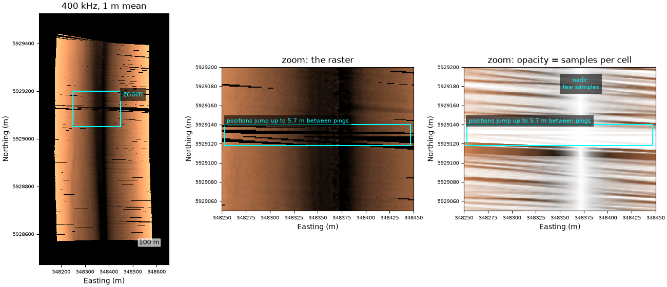
plot_grid_coverage() draws the same raster with each cell’s opacity set by its sample count (n_contributing_samples), full at the 95th percentile. Below, the whole 400 kHz line at 1 m with the default mean, and a 200 m by 150 m zoom. It is a check on the grid, not a map product.

mean_1m = grid_channel(ds400, resolution_m=1.0)
counts = mean_1m.dataset["n_contributing_samples"].values
print("samples per cell with data, 5th, 50th and 95th percentile:", np.percentile(counts[counts > 0], [5, 50, 95]))

zx, zy = (348250.0, 348450.0), (5929050.0, 5929200.0)
fig, axes = plt.subplots(1, 3, figsize=(13, 5.6), width_ratios=[0.8, 1, 1], constrained_layout=True)
plot_gridded_raster(mean_1m, fig=fig, ax=axes[0], cmap="copper", vmin_pct=2, vmax_pct=98, show_colorbar=False,
                    title="400 kHz, 1 m mean")
axes[0].add_patch(Rectangle((zx[0], zy[0]), zx[1] - zx[0], zy[1] - zy[0], fill=False, ec="cyan", lw=1.5))
axes[0].text(zx[1] + 10, zy[1], "zoom", color="cyan", va="top", bbox=dict(fc="black", alpha=0.6, lw=0))
plot_gridded_raster(mean_1m, fig=fig, ax=axes[1], cmap="copper", vmin_pct=2, vmax_pct=98, show_colorbar=False,
                    show_scale_bar=False, title="zoom: the raster")
plot_grid_coverage(mean_1m, fig=fig, ax=axes[2], cmap="copper", vmin_pct=2, vmax_pct=98,
                   title="zoom: opacity = samples per cell")
for ax in axes:
    ax.ticklabel_format(useOffset=False, style="plain")
    ax.tick_params(labelsize=7)
for ax in axes[1:]:
    ax.set(xlim=zx, ylim=zy)
    ax.add_patch(Rectangle((zx[0] + 3, 5929118), 194, 22, fill=False, ec="cyan", lw=1.5))
    ax.text(zx[0] + 5, 5929142, "positions jump up to 5.7 m between pings", color="cyan", fontsize=8,
            bbox=dict(fc="black", alpha=0.6, lw=0))
axes[2].text(348372, 5929190, "nadir:\nfew samples", color="cyan", fontsize=8, ha="center", va="top",
             bbox=dict(fc="black", alpha=0.6, lw=0))
fig.savefig(out / "grid_coverage.png", dpi=150)

samples per cell with data, 5th, 50th and 95th percentile: [ 33. 160. 444.]

Reading the result

Near nadir each sample covers more ground, so cells there hold few samples and fade out. The slanted bands are where successive pings fan together or apart as the heading wanders: the same patch of seabed gets more or fewer pings, not misplaced data. A jump in the positions leaves a strip with no samples at all, which only a larger search radius (idw, 4 m, above) bridges.