sidescanpy#
Read, correct, grid and export sidescan sonar data.
sidescanpy converts EdgeTech JSF, Klein SDF and XTF surveys into one
xarray-based model stored as .ss.h5, then corrects it (TVG, ground
range, georeferencing), slices it, grids it to rasters and GeoTIFF, and
builds COCO/YOLO training datasets from target catalogs. Small analysis
functions measure a dataset’s units, nadir, usable range and TVG state.
Beta
Until 1.0, any 0.x release may change the .ss.h5 file format, the
API and the CLI. Keep your raw sonar files, pin the version you use,
and expect to re-convert .ss.h5 files after an upgrade. See
Stability.
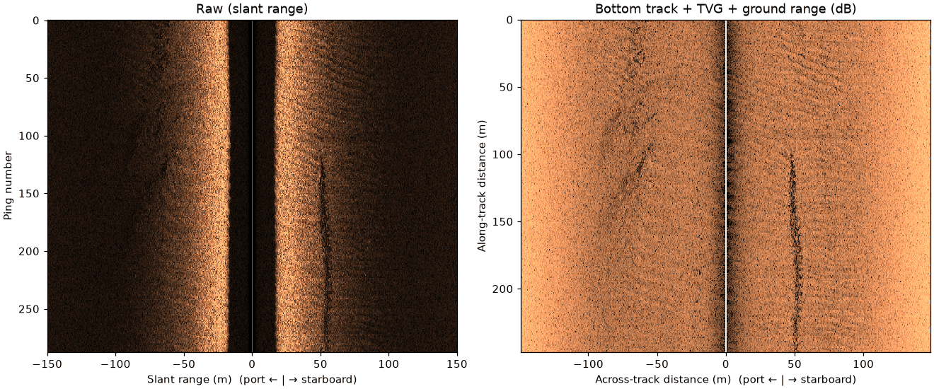
A public EdgeTech recording, raw (left) and after the bottom track, TVG and slant-to-ground-range steps (right). Code and data: Correct a line.
Quickstart#
from sidescanpy import datasets
from sidescanpy.grids import grid_channel, to_geotiff
from sidescanpy.io import read_and_convert
from sidescanpy.io.hdf5 import write_survey
from sidescanpy.processing import (
    apply_tvg,
    compute_geometric_ranges,
    compute_georeferencing,
    interpolate_aux_onto_pings,
)

# A public Benthos XTF line; any JSF, SDF or XTF path works the same way.
path = datasets.fetch("jncc_mid_irish_sea_MIS11_0.xtf")
survey = read_and_convert([path], fmt="xtf")

survey = interpolate_aux_onto_pings(survey)   # navigation onto the pings
survey = apply_tvg(survey)                    # time-varying gain
survey = compute_geometric_ranges(survey)     # slant to ground range
survey = compute_georeferencing(survey)       # latitude and longitude per sample
write_survey(survey, "MIS11_0.ss.h5")

# Grid one frequency at 1 m and write a GeoTIFF (needs the geo extra).
raster = grid_channel(survey.get_frequency("hz_400000").dataset, resolution_m=1.0)
to_geotiff(raster, "MIS11_0_400khz.tif")
Install covers the install and its extras. Getting started walks through this code step by step, with the output of each step.
Citing#
If you use sidescanpy in your work, please cite it: Shomberg, R. sidescanpy: read, correct, grid and export sidescan sonar data. Zenodo. doi:10.5281/zenodo.24121873. This concept DOI always resolves to the latest release; each release on Zenodo also has its own version DOI.
Where to go next#
Start here: Install, Getting started.
Examples: real data, code and results, all on openly licensed recordings you can download, plus target recognition step by step.
Theory: why sidescan looks the way it does: the physics behind each processing step, measured on the same public recordings.
Example data: every public recording the Examples and Theory pages use, with its source, size and licence, and how
sidescanpy.datasets.fetchdownloads it.Public datasets: openly published sidescan archives and whether sidescanpy reads them, with a sample figure for each one it does.
Guide: Building a workflow, Data model, Processing, Gridding, Targets and datasets, Analysis, Visualization, Command line, Logging, Limitations.
Data format: the format every reader converts into: the .ss.h5 file and NetCDF for one frequency. A draft, open for comment.
Source formats: overview, EdgeTech JSF, Klein SDF, XTF, and adding a source format.
Reference: API reference, one page per module, generated from the docstrings.