Four passes over one wreck: native and north-up

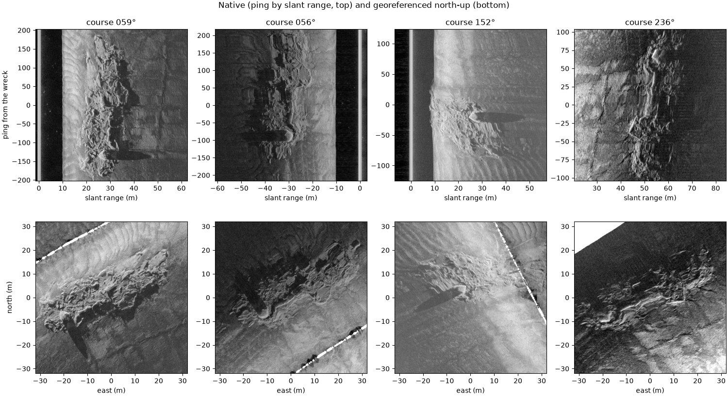
The same wreck seen on four lines run in three directions. In the native view (ping by slant range) each pass looks different: the wreck is lit from a different side, its shadow points away from the track, and near nadir it is compressed in range. Georeferenced north-up onto one map grid, the four views agree on where the wreck is and what shape it has, but only once the navigation is right. Here that takes four steps:

1. Ship positions. These files record no heading (0 throughout). The recorder still offset its towfish position from the ship by a tow-point offset rotated by that heading, so on every line it points south whatever the course. The XTF reader detects this and uses the ship positions instead, recording the offset as the tow point.

2. Smoothed navigation. The positions jump back by 1 to 3 m at every GPS fix (see Eight wrecks at one scale); smooth_navigation() removes the jumps.

3. Course as heading. With no compass, course_over_ground() gives the direction each ping looks across.

4. Layback. The towfish trails the ship by the tow-point offset plus the cable. The cable length was not recorded, so the cable layback here (27.5 m, beyond the 12.5 m tow point) was found from two pairs of passes run in opposite directions: with only the tow point applied they place the wreck 53 to 57 m apart along the track, twice the missing layback (Where the towfish is: navigation and layback measures it).

Data: BGS London Gateway, Klein 3000 at 400 kHz, Open Government Licence v3.0, contains data supplied by UKRI (see Example data).

Usage: python examples/gallery/plot_four_passes.py [output_dir]

# 2026 rshomberg@uri.edu

import sys
from pathlib import Path

import matplotlib.pyplot as plt
import numpy as np
from pyproj import Transformer

from sidescanpy import datasets
from sidescanpy.export.georef_window import extract_georef_window
from sidescanpy.export.windows.levels import with_db_var
from sidescanpy.io import read_and_convert
from sidescanpy.log import configure_logging
from sidescanpy.processing import (
    altitude_from_bottom_track,
    apply_layback,
    compute_geometric_ranges,
    compute_georeferencing,
    course_over_ground,
    interpolate_aux_onto_pings,
    smooth_navigation,
)
from sidescanpy.processing.navigation import along_track_distance_m

out = Path(sys.argv[1]) if len(sys.argv) > 1 else Path(".")
out.mkdir(parents=True, exist_ok=True)
configure_logging("ERROR")

LINES = ["bgs_london_gateway_dynamo_78.xtf", "bgs_london_gateway_dynamo_86.xtf",
         "bgs_london_gateway_dynamo_88.xtf", "bgs_london_gateway_dynamo_85.xtf"]
LAYBACK_M = 27.5
WINDOW_M, CELL_M = 64.0, 0.15

# The catalogued wreck position (UTM zone 31N), moved to the middle of the
# wreck as these passes place it.
east, north = datasets.BGS_LONDON_GATEWAY_WRECKS["Dynamo"]
to_lonlat = Transformer.from_crs(32631, 4326, always_xy=True)
wreck_lon, wreck_lat = to_lonlat.transform(east - 4.0, north + 6.0)

What the reader found

position_source says the positions are the ship’s, and the reason gives the offset the recorder had applied; tow_point_aft_m and tow_point_starboard_m carry it to the layback step.

survey = read_and_convert([datasets.fetch(LINES[0])], fmt="xtf", nav_crs="EPSG:32631")
attrs = survey.get_frequency("hz_400000").dataset.attrs
print(attrs["position_source"])
print(attrs["position_source_reason"].split("). ", 1)[1])

ship
bgs_london_gateway_dynamo_78.xtf: Sensor is Ship shifted -1.80 m east, -12.50 m north on every ping, whatever the course: an offset rotated by heading 0 (no heading recorded), so Ship positions are used; tow point 12.50 m aft, -1.80 m starboard

One pass, step by step

The steps in order, then the pings within 70 m of the wreck, then ground range and a latitude and longitude for every sample. No TVG: the recorder applied its own, so the samples are only converted to dB.

def georeferenced_pass(name):
    survey = read_and_convert([datasets.fetch(name)], fmt="xtf", nav_crs="EPSG:32631")
    survey = smooth_navigation(interpolate_aux_onto_pings(survey), window_s=5.0)
    ds = survey.get_frequency("hz_400000").dataset.load()
    ds = ds.assign(heading_deg=("ping", course_over_ground(ds, half_window_s=15.0)))
    ds = apply_layback(ds, layback_m=LAYBACK_M)
    closest = int(np.nanargmin(np.hypot(ds["latitude"].values - wreck_lat,
                                        (ds["longitude"].values - wreck_lon) * np.cos(np.radians(wreck_lat)))))
    ds = ds.isel(ping=slice(max(closest - 450, 0), closest + 450))
    ds = compute_georeferencing(compute_geometric_ranges(altitude_from_bottom_track(ds)))
    return with_db_var(ds)


passes = [georeferenced_pass(name) for name in LINES]

The native view

Ping by signed slant range (port negative), the samples as recorded. Each crop is centred on the sample nearest the wreck centre, 64 m of range across and the pings covering 64 m along track.

def native_crop(ds):
    lat, lon = ds["latitude_per_sample"].values, ds["longitude_per_sample"].values
    dist = np.hypot(lat - wreck_lat, (lon - wreck_lon) * np.cos(np.radians(wreck_lat)))
    ping, channel, sample = np.unravel_index(np.nanargmin(dist), dist.shape)
    db = ds["backscatter_db"].values
    swath = np.concatenate([db[:, 0, ::-1], db[:, 1]], axis=1)
    slant = ds["slant_range_m"].values[ping, 1]
    signed = np.concatenate([-slant[::-1], slant])
    centre = slant[sample] * (1 if channel == 1 else -1)
    cols = np.flatnonzero(np.abs(signed - centre) <= WINDOW_M / 2)
    along = along_track_distance_m(ds, fill_nav_stalls=True) - along_track_distance_m(ds, fill_nav_stalls=True)[ping]
    rows = np.flatnonzero(np.abs(along) <= WINDOW_M / 2)
    course = float(ds["heading_deg"].values[ping])
    return swath[np.ix_(rows, cols)], (signed[cols[0]], signed[cols[-1]], rows[0] - ping, rows[-1] - ping), course


natives = [native_crop(ds) for ds in passes]

The north-up view

The same pings gridded onto one 64 m map window at 0.15 m cells, by linear interpolation between the samples (scipy griddata).

size_px = int(round(WINDOW_M / CELL_M))
maps = [extract_georef_window(ds, size_px, resolution_m=CELL_M, center_lat=wreck_lat, center_lon=wreck_lon,
                              backscatter_var="backscatter_db", interp_method="linear")[0].backscatter
        for ds in passes]

half = WINDOW_M / 2
fig, axes = plt.subplots(2, 4, figsize=(15, 8.2), constrained_layout=True)
for k, ((crop, extent, course), grid) in enumerate(zip(natives, maps)):
    lo, hi = np.nanpercentile(np.concatenate([crop[np.isfinite(crop)], grid[np.isfinite(grid)]]), [1, 99.7])
    ax = axes[0, k]
    ax.imshow(crop, cmap="gray", vmin=lo, vmax=hi, origin="lower", aspect="auto", extent=extent)
    ax.set_box_aspect(1)
    ax.set_title(f"course {course:03.0f}°")
    ax.set_xlabel("slant range (m)")
    ax = axes[1, k]
    ax.imshow(grid, cmap="gray", vmin=lo, vmax=hi, origin="lower", extent=[-half, half, -half, half])
    ax.set_facecolor("white")
    ax.set_xlabel("east (m)")
axes[0, 0].set_ylabel("ping from the wreck")
axes[1, 0].set_ylabel("north (m)")
fig.suptitle("Native (ping by slant range, top) and georeferenced north-up (bottom)")
fig.savefig(out / "four_passes.png", dpi=200)

Reading the result

On the map the four passes put the hull in the same place to within a few meters. What is left has three sources. A tidal current set the towfish sideways off the ship’s track on the south-east line (the passes made 1.35 m/s over the ground running north-east and 2.65 m/s running south-west, so about 0.65 m/s of current), and a layback only moves a pass along its course. The layback is one value for all four lines, while the real one varies a little from line to line. And the course stands in for the heading. The shadows point away from each track, so each pass shows a different side of the wreck: a mosaic of all four would show more of it than any one.

Why the 152° pass looks different

Same wreck, different geometry. The other passes run along the hull; this one crosses it end-on, close under the towfish (about 10 m slant range), where shadows are short and the recorder’s gain makes the seabed bright. Its track is on the other side, so the shadows fall the other way.