The sonar equation and time-varying gain

The sonar equation keeps the books on an echo in decibels. The echo level EL the receiver sees is the source level SL the transducer sends, less the transmission loss TL on the way out and again on the way back, plus the backscatter strength BS of whatever returned the sound:

\[EL = SL - 2 \, TL + BS\]

One way, the sound spreads over a sphere and seawater absorbs part of it, alpha dB per meter:

\[TL = 20 \log_{10} R + \alpha R\]

so the echo of a single small target falls as 40 log10 R + 2 alpha R with slant range R.

The seabed is not a single target. Its backscatter strength is a strength per square meter, S_b, times the patch of seabed the pulse lights at one time, A:

\[BS = S_b + 10 \log_{10} A\]

Along track the patch is as wide as the beam, R theta for a beam of horizontal width theta; across track it is set by the pulse and, at the low grazing angles of sidescan, hardly changes with range. So A grows in proportion to R, which wins back 10 log10 R, and the seabed echo falls about

\[30 \log_{10} R + 2 \alpha R\]

(Tamsett, 2017, doi:10.3390/jmse5040054). Fisheries echosounders, which measure fish spread through a volume, use 20 log10 R for the same reason: the lit volume grows as R^2.

The levels in a sidescan file are relative (Echo amplitude and decibels), so SL, the receiver gain and the absolute S_b are one unknown constant. Only how the level changes with range matters. Time-varying gain (TVG) adds back the modelled loss, n log10 R + 2 alpha R, so a uniform seabed comes out at the same level at all ranges. Many recorders apply some TVG in hardware and do not record which, so the right model is fitted to each recording rather than assumed. Absorption is computed with Francois and Garrison (1982), J. Acoust. Soc. Am. 72(3) 896-907 and 72(6) 1879-1890.

TVG corrects the loss along the path only. What it leaves behind is the transducer’s beam pattern and the way the seabed scatters less at low grazing angles (Lambert’s law: S_b falls with the square of the sine of the grazing angle). sidescanpy’s empirical range correction flattens those.

Data: JNCC Wight-Barfleur Reef, EdgeTech JSF (Open Government Licence v3.0); USGS Grand Bay, Klein XTF (public domain); BGS London Gateway, Klein 3000 XTF (Open Government Licence v3.0, contains data supplied by UKRI) (see Example data).

Usage: python examples/theory/plot_sonar_equation_and_tvg.py [output_dir]

# 2026 rshomberg@uri.edu

import sys
from pathlib import Path

import matplotlib.pyplot as plt
import numpy as np
from matplotlib.patches import Rectangle

from sidescanpy import analysis, datasets
from sidescanpy.io import read_and_convert
from sidescanpy.log import configure_logging
from sidescanpy.processing import (
    altitude_from_bottom_track,
    apply_tvg,
    compute_geometric_ranges,
    slice_by_range,
)
from sidescanpy.processing.radiometric import (
    center_frequency_hz,
    francois_garrison_absorption_db_per_m,
)
from sidescanpy.viz.tvg import plot_tvg_fit

out = Path(sys.argv[1]) if len(sys.argv) > 1 else Path(".")
out.mkdir(parents=True, exist_ok=True)
configure_logging("ERROR")

Spreading laws and absorption

Two-way loss relative to its value at 10 m, for the three spreading laws alone and for 30 log R with absorption at three frequencies (Francois-Garrison, default water: 10 C, salinity 35, 10 m depth, pH 8). The curves differ most at short range, where log10 R changes fastest; absorption takes over at long range and high frequency.

R = np.linspace(2, 200, 400)
R_REF = 10.0
fig, ax = plt.subplots(figsize=(9, 5), constrained_layout=True)
for n, ls in ((20, ":"), (30, "-"), (40, "--")):
    ax.plot(R, n * np.log10(R / R_REF), color="k", ls=ls, lw=1.4, label=f"{n} log R")
for f_khz, colour in ((100, "C2"), (400, "C1"), (548, "C3")):
    a = francois_garrison_absorption_db_per_m(f_khz * 1e3)
    ax.plot(R, 30 * np.log10(R / R_REF) + 2 * a * (R - R_REF), color=colour, lw=2,
            label=f"30 log R + 2 alpha R, {f_khz} kHz (alpha {1000 * a:.0f} dB/km)")
    print(f"{f_khz} kHz: alpha = {a:.4f} dB/m; two-way absorption from 10 to 100 m: 2 x {a:.4f} x 90 = "
          f"{2 * a * 90:.1f} dB")
print(f"spreading from 10 to 100 m: 20 log R {20:.0f} dB, 30 log R {30:.0f} dB, 40 log R {40:.0f} dB")
ax.set_xlim(0, 200)
ax.set_ylim(-25, 110)
ax.set_xlabel("slant range R (m)")
ax.set_ylabel("two-way loss relative to 10 m (dB)")
ax.set_title("What TVG must add back: spreading plus absorption", loc="left")
ax.grid(alpha=0.3)
ax.legend(loc="upper left", fontsize=9)
fig.savefig(out / "sonar_equation_and_tvg_laws.png", dpi=150)

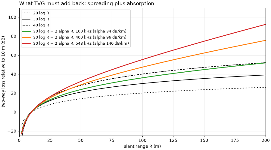
100 kHz: alpha = 0.0336 dB/m; two-way absorption from 10 to 100 m: 2 x 0.0336 x 90 = 6.0 dB
400 kHz: alpha = 0.0960 dB/m; two-way absorption from 10 to 100 m: 2 x 0.0960 x 90 = 17.3 dB
548 kHz: alpha = 0.1404 dB/m; two-way absorption from 10 to 100 m: 2 x 0.1404 x 90 = 25.3 dB
spreading from 10 to 100 m: 20 log R 20 dB, 30 log R 30 dB, 40 log R 40 dB

Three recordings

The high frequency of the Wight-Barfleur line (a chirp from 521 to 574 kHz, center 548 kHz, sidescanpy key hz_521000, named by the start of the sweep; labels use the center. The JSF records no altitude, so it comes from the first seabed echo), a Klein line from the shallow Grand Bay estuary (100 kHz) and a London Gateway line (Klein 3000, 400 kHz) whose recorder applied its own TVG. Incomplete pings are dropped.

RECORDINGS = {
    "Wight-Barfleur, 548 kHz": ("jncc_wight_barfleur_20130321174522.jsf", {"fmt": "jsf"}, "hz_521000"),
    "Grand Bay, 100 kHz": ("usgs_grand_bay_150602205800.xtf", {"fmt": "xtf"}, "hz_100000"),
    "London Gateway, 400 kHz": ("bgs_london_gateway_dynamo_88.xtf", {"fmt": "xtf", "nav_crs": "EPSG:32631"},
                                "hz_400000"),
}
lines = {}
for label, (name, kwargs, key) in RECORDINGS.items():
    ds = read_and_convert([datasets.fetch(name)], **kwargs).get_frequency(key).dataset.load()
    ds = ds.isel(ping=np.isfinite(ds["backscatter_intensity"].values).all(axis=(1, 2)))
    ds = compute_geometric_ranges(altitude_from_bottom_track(ds))
    alpha = francois_garrison_absorption_db_per_m(center_frequency_hz(ds))
    lines[label] = dict(ds=ds, alpha=alpha, altitude=float(np.nanmedian(ds["altitude_m"].values)))
    print(f"{label}: {ds.sizes['ping']} pings, altitude {lines[label]['altitude']:.1f} m (median), "
          f"{float(ds['slant_range_m'].max()):.0f} m recorded, alpha {1000 * alpha:.1f} dB/km")

Wight-Barfleur, 548 kHz: 287 pings, altitude 17.5 m (median), 200 m recorded, alpha 140.2 dB/km
Grand Bay, 100 kHz: 297 pings, altitude 1.7 m (median), 100 m recorded, alpha 33.6 dB/km
London Gateway, 400 kHz: 1234 pings, altitude 9.4 m (median), 84 m recorded, alpha 96.0 dB/km

The median level against range

This page fits with the library: fit_tvg_models() measures the profile, picks the window and fits the models, and check_tvg() applies the result.

The profile: for each line, all samples beyond the altitude (past the water column), both sides, binned by slant range in 1 m bins; the median of each bin in dB re 1 recorded unit (median_level_profile()). The two Klein files store whole numbers, so each sample is first spread evenly over its unit interval (a fixed random offset between -0.5 and 0.5); without it the medians stick to whole numbers and the profile has steps.

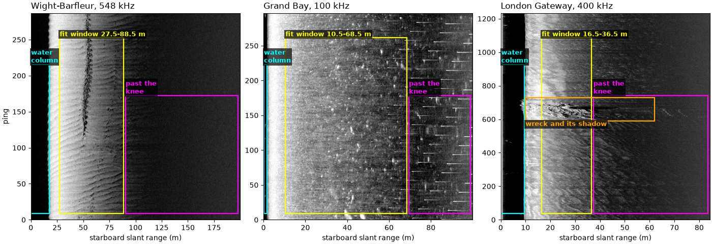
The fit window starts 5 m past the profile’s peak (inside the peak the beam pattern dominates) and ends at the noise knee, the first range past the peak where the level comes within 3 dB of its lowest value (find_noise_knee()). Beyond the knee the level is noise, which no spreading law describes.

The models: L(R) = L0 - n log10 R - k 2 alpha R with n = 20, 30 or 40 and absorption off (k = 0) or on (k = 1). Each has only L0 free, the unknown constant of the sonar equation. A seventh lets n float too, with absorption on. The RMS residual over the fit window ranks them.

SPREADING = (20.0, 30.0, 40.0)
for label, line in lines.items():
    line["fit"] = fit = analysis.fit_tvg_models(line["ds"], spreading=SPREADING)
    line["window"] = fit.window_m
    peak_db = float(np.interp(fit.peak_m, fit.range_m, fit.level_db))
    print(f"{label}: peak {peak_db:.1f} dB at {fit.peak_m:.1f} m; lowest {peak_db - fit.contrast_db:.1f} dB; "
          f"knee {fit.knee_m:.1f} m; fit window {fit.window_m[0]:.1f} to {fit.window_m[1]:.1f} m")

Wight-Barfleur, 548 kHz: peak 44.6 dB at 22.5 m; lowest 8.0 dB; knee 88.5 m; fit window 27.5 to 88.5 m
Grand Bay, 100 kHz: peak 48.2 dB at 5.5 m; lowest 22.4 dB; knee 68.5 m; fit window 10.5 to 68.5 m
London Gateway, 400 kHz: peak 49.2 dB at 11.5 m; lowest 29.9 dB; knee 36.5 m; fit window 16.5 to 36.5 m

The figure shows each line’s starboard side as recorded, with the parts of the image this section uses boxed: the water column (left out), the fit window, and the range past the noise knee, where the level no longer falls.

def label_box(ax, x0, x1, y0, y1, text, colour="cyan", where="above", fontsize=9):
    """Outline a feature with a rectangle and name it."""
    ax.add_patch(Rectangle((x0, y0), x1 - x0, y1 - y0, fill=False, ec=colour, lw=1.6))
    y = y1 if where == "above" else y0
    ax.text(x0, y, text, color=colour, fontsize=fontsize, fontweight="bold",
            va="bottom" if where == "above" else "top", ha="left",
            bbox=dict(boxstyle="square,pad=0.15", fc="black", ec="none", alpha=0.7))


fig, axes = plt.subplots(1, 3, figsize=(14, 4.8), constrained_layout=True)
for ax, (label, line) in zip(axes, lines.items()):
    ds = line["ds"]
    slant_row = ds["slant_range_m"].values[0, 1]
    n = max(1, int(round(0.1 / float(slant_row[1] - slant_row[0]))))
    amp = ds["backscatter_intensity"].values[:, 1].astype(np.float64)
    keep = (amp.shape[1] // n) * n
    img = 20 * np.log10(amp[:, :keep].reshape(amp.shape[0], -1, n).mean(axis=2) + 1e-3)
    r_end = float(slant_row[keep - 1])
    n_p = img.shape[0]
    lo, hi = np.percentile(img[:, img.shape[1] // 10:], [2, 99.5])
    ax.imshow(img, cmap="gray", vmin=lo, vmax=hi, origin="lower", aspect="auto", extent=[0, r_end, 0, n_p])
    w0, w1 = line["window"]
    label_box(ax, 0.2, line["altitude"], 0.03 * n_p, 0.75 * n_p, "water\ncolumn", colour="cyan")
    label_box(ax, w0, w1, 0.03 * n_p, 0.88 * n_p, f"fit window {w0:.1f}-{w1:.1f} m", colour="yellow")
    if w1 < 0.97 * r_end:
        label_box(ax, w1 + 0.01 * r_end, 0.99 * r_end, 0.03 * n_p, 0.6 * n_p, "past the\nknee", colour="magenta")
    if label.startswith("London Gateway"):
        label_box(ax, 10, 62, 590, 730, "wreck and its shadow", colour="orange", where="below")
    ax.set_xlabel("starboard slant range (m)")
    ax.set_title(label, loc="left")
axes[0].set_ylabel("ping")
fig.savefig(out / "sonar_equation_and_tvg_windows.png", dpi=150)

Fitting the spreading law

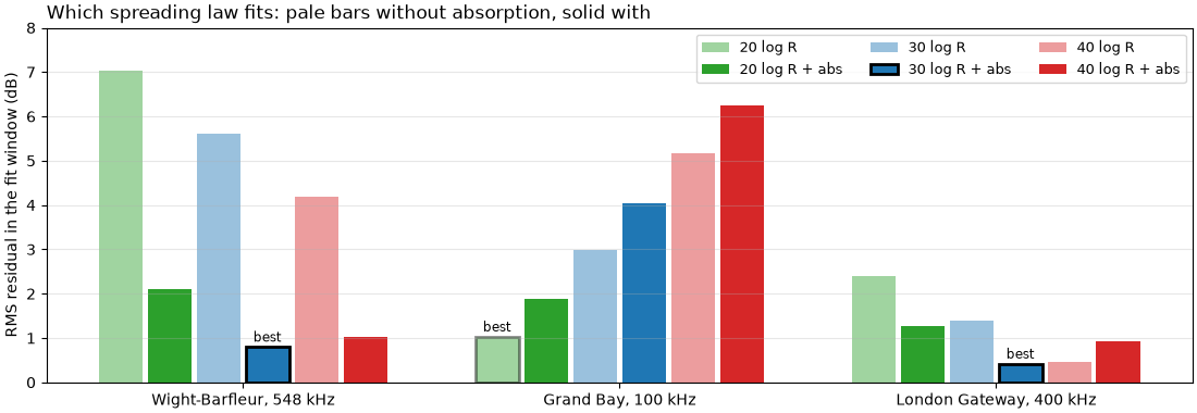
The fit results, line by line: the RMS residual of each model, the best and the runner-up, the free n, and each side fitted alone on the same window.

MODELS = [analysis.tvg_model_name(n, k) for n in SPREADING for k in (False, True)]
for label, line in lines.items():
    fit = line["fit"]
    table = ", ".join(f"{name} {fit.models[name].rms_db:.2f}" for name in MODELS)
    print(f"{label} ({fit.n_bins} bins): RMS residual (dB): {table}")
    print(f"   best {fit.best} ({fit.best_model.rms_db:.2f} dB), next {fit.runner_up} "
          f"({fit.runner_up_model.rms_db:.2f} dB); free fit with absorption: n = {fit.free_n:.1f}, "
          f"RMS {fit.free_n_rms_db:.2f} dB")
    per_side = "; ".join(f"{sf.side} {sf.best} ({sf.rms_db:.2f} dB)" for sf in fit.side_best)
    print(f"   each side alone, same window: {per_side}")
    w0, w1 = fit.window_m
    fall = np.interp(w0, fit.range_m, fit.level_db) - np.interp(w1, fit.range_m, fit.level_db)
    alpha = fit.absorption_db_per_m
    print(f"   the level falls {fall:.1f} dB from {w0:.1f} to {w1:.1f} m; 30 log R + abs predicts "
          f"30 log10({w1 / w0:.2f}) + 2 x {alpha:.4f} x {w1 - w0:.0f} = "
          f"{30 * np.log10(w1 / w0) + 2 * alpha * (w1 - w0):.1f} dB")

Wight-Barfleur, 548 kHz (62 bins): RMS residual (dB): 20 log R 7.03, 20 log R + abs 2.10, 30 log R 5.60, 30 log R + abs 0.80, 40 log R 4.18, 40 log R + abs 1.02
   best 30 log R + abs (0.80 dB), next 40 log R + abs (1.02 dB); free fit with absorption: n = 34.0, RMS 0.55 dB
   each side alone, same window: port 40 log R + abs (0.64 dB); starboard 30 log R + abs (1.04 dB)
   the level falls 32.6 dB from 27.5 to 88.5 m; 30 log R + abs predicts 30 log10(3.22) + 2 x 0.1402 x 61 = 32.3 dB
Grand Bay, 100 kHz (59 bins): RMS residual (dB): 20 log R 1.03, 20 log R + abs 1.89, 30 log R 2.99, 30 log R + abs 4.04, 40 log R 5.16, 40 log R + abs 6.24
   best 20 log R (1.03 dB), next 20 log R + abs (1.89 dB); free fit with absorption: n = 12.0, RMS 0.63 dB
   each side alone, same window: port 20 log R (4.00 dB); starboard 20 log R + abs (0.89 dB)
   the level falls 16.1 dB from 10.5 to 68.5 m; 30 log R + abs predicts 30 log10(6.52) + 2 x 0.0336 x 58 = 28.3 dB
London Gateway, 400 kHz (21 bins): RMS residual (dB): 20 log R 2.40, 20 log R + abs 1.28, 30 log R 1.39, 30 log R + abs 0.42, 40 log R 0.45, 40 log R + abs 0.92
   best 30 log R + abs (0.42 dB), next 40 log R (0.45 dB); free fit with absorption: n = 31.9, RMS 0.37 dB
   each side alone, same window: port 40 log R (0.37 dB); starboard 30 log R + abs (0.55 dB)
   the level falls 14.3 dB from 16.5 to 36.5 m; 30 log R + abs predicts 30 log10(2.21) + 2 x 0.0960 x 20 = 14.2 dB

The figure is the table above as bars: the RMS residual of each fixed model on each line, best model outlined. Lower is better.

COLOURS = {20.0: "C2", 30.0: "C0", 40.0: "C3"}
fig, ax = plt.subplots(figsize=(11, 3.8), constrained_layout=True)
width = 0.13
for j, name in enumerate(MODELS):
    for i, line in enumerate(lines.values()):
        model = line["fit"].models[name]
        best = name == line["fit"].best
        ax.bar(i + (j - 2.5) * width, model.rms_db, width * 0.9, color=COLOURS[model.spreading_loss_db],
               alpha=1 if model.absorption_db_per_m > 0 else 0.45, ec="k" if best else "none", lw=2 if best else 0,
               label=name if i == 0 else None)
        rms = model.rms_db
        if best:
            ax.text(i + (j - 2.5) * width, rms + 0.12, "best", ha="center", fontsize=8.5)
ax.set_xticks(range(len(lines)), labels=list(lines))
ax.set_ylabel("RMS residual in the fit window (dB)")
ax.set_title("Which spreading law fits: pale bars without absorption, solid with", loc="left")
ax.grid(alpha=0.3, axis="y")
ax.legend(ncol=3, fontsize=9, loc="upper right")
ax.set_ylim(0, 8)
fig.savefig(out / "sonar_equation_and_tvg_rms.png", dpi=150)

Applying the TVG

A good fit is a hypothesis. To test it, check_tvg() crops each line at its noise knee with slice_by_range() (beyond it TVG would only amplify noise), corrects it with apply_tvg() using its own best model, and bins the result as the fit did. If the model is right the corrected median level is flat across the fit window.

for label, line in lines.items():
    fit = line["fit"]
    line["check"] = check = analysis.check_tvg(line["ds"], fit.tvg_params, fit.window_m)
    print(f"{label}: after TVG with {check.model_name}: spread {check.spread_db:.2f} dB, "
          f"trend {check.trend_db_per_10m:+.2f} dB per 10 m across the window")
for label, (n, with_abs) in (("Wight-Barfleur, 548 kHz", (20.0, True)), ("Grand Bay, 100 kHz", (30.0, True))):
    fit = lines[label]["fit"]
    params = {"spreading_loss_db": n, "absorption_db_per_m": fit.absorption_db_per_m if with_abs else 0.0}
    wrong = analysis.check_tvg(lines[label]["ds"], params, fit.window_m)
    print(f"{label} with {wrong.model_name} instead: trend {wrong.trend_db_per_10m:+.2f} dB per 10 m, "
          f"{wrong.end_to_end_db:+.1f} dB from one end of the window to the other")

Wight-Barfleur, 548 kHz: after TVG with 30 log R + abs: spread 0.80 dB, trend -0.32 dB per 10 m across the window
Grand Bay, 100 kHz: after TVG with 20 log R: spread 1.02 dB, trend +0.31 dB per 10 m across the window
London Gateway, 400 kHz: after TVG with 30 log R + abs: spread 0.42 dB, trend -0.28 dB per 10 m across the window
Wight-Barfleur, 548 kHz with 20 log R + abs instead: trend -1.11 dB per 10 m, -5.5 dB from one end of the window to the other
Grand Bay, 100 kHz with 30 log R + abs instead: trend +2.25 dB per 10 m, +12.7 dB from one end of the window to the other

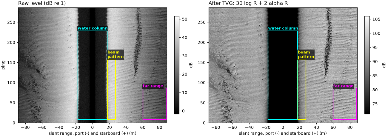
The Wight-Barfleur swath before and after

The raw level in dB and the same pings after apply_tvg() with 30 log R and absorption, both sides, cropped at the noise knee. Boxed on starboard: the water column, the stretch between the water column and the start of the fit window where the beam pattern still shapes the level, and the far range, dark before TVG and as bright as the near range after it. Each panel’s gray scale is stretched over its seabed samples only.

wb = lines["Wight-Barfleur, 548 kHz"]
cropped = slice_by_range(wb["ds"], max_m=wb["window"][1])
raw = cropped["backscatter_intensity"].values
after = apply_tvg(cropped, wb["fit"].tvg_params)["backscatter_intensity"].values
knee = wb["window"][1]
fig, axes = plt.subplots(1, 2, figsize=(13, 4.6), constrained_layout=True)
for ax, data, title in ((axes[0], 20 * np.log10(np.maximum(raw, 1e-6)), "Raw level (dB re 1)"),
                        (axes[1], after, "After TVG: 30 log R + 2 alpha R")):
    swath = np.concatenate([data[:, 0, ::-1], data[:, 1]], axis=1)
    # Stretch on the seabed only: the dark water column would otherwise
    # take half the gray scale and wash the seabed out.
    signed = np.linspace(-knee, knee, swath.shape[1])
    seabed = swath[:, np.abs(signed) > wb["altitude"] + 1.0]
    lo, hi = np.percentile(seabed[np.isfinite(seabed) & (seabed > -100)], [1, 99.5])
    im = ax.imshow(swath, cmap="gray", vmin=lo, vmax=hi, aspect="auto", origin="lower",
                   extent=[-knee, knee, 0, swath.shape[0]])
    ax.set_title(title, loc="left")
    ax.set_xlabel("slant range, port (-) and starboard (+) (m)")
    fig.colorbar(im, ax=ax, label="dB", shrink=0.85)
    n_p = swath.shape[0]
    label_box(ax, -wb["altitude"], wb["altitude"], 0.03 * n_p, 0.8 * n_p, "water column", colour="cyan")
for ax in axes:
    label_box(ax, wb["altitude"] + 0.5, wb["window"][0], 0.03 * n_p, 0.55 * n_p, "beam\npattern",
              colour="yellow")
    label_box(ax, 60, knee - 0.5, 0.03 * n_p, 0.3 * n_p, "far range", colour="magenta")
axes[0].set_ylabel("ping")
fig.savefig(out / "sonar_equation_and_tvg_swath.png", dpi=150)

Fit, apply, check

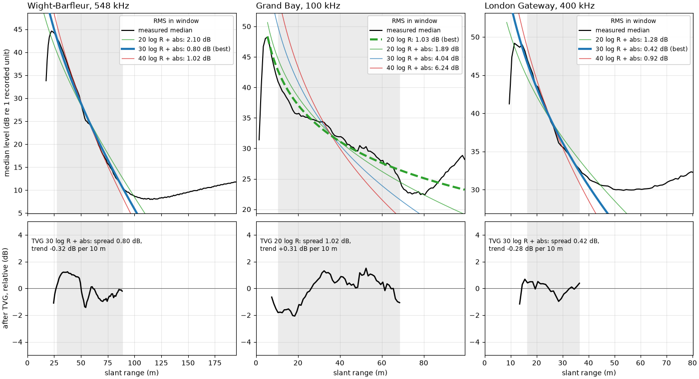
Each column is the library’s own figure, plot_tvg_fit(), drawn from the fit_tvg_models() and check_tvg() results above. Top: the median level against slant range (black) for each line, with the 20, 30 and 40 log R models with absorption anchored to it, the best model (thick), and the fit window (shaded). Bottom: the median level after apply_tvg() with that best model, relative to its mean in the window. Flat means the model holds.

fig, axes = plt.subplots(2, 3, figsize=(14, 7.6), height_ratios=[1.5, 1], sharex="col", constrained_layout=True)
for col, (label, line) in enumerate(lines.items()):
    plot_tvg_fit(line["fit"], line["check"], ax=axes[0, col], ax_check=axes[1, col], title=label)
    if col:
        axes[0, col].set_ylabel("")
        axes[1, col].set_ylabel("")
fig.savefig(out / "sonar_equation_and_tvg.png", dpi=150)

Reading the result

Each line needs its own model. Over its fit window (27.5 to 88.5 m) the Wight-Barfleur high frequency falls 32.6 dB, and 30 log R with absorption predicts 32.3 dB: 30 log10(88.5 / 27.5) + 2 x 0.1402 x 61 = 32.3. That model fits best (0.80 dB RMS), with 40 log R plus absorption close behind (1.02 dB); letting n float gives 34.0 at 0.55 dB, between the two. The Grand Bay line falls only 16.1 dB over 10.5 to 68.5 m, where 30 log R with absorption predicts 28.3 dB. Its best fixed model is 20 log R without absorption (1.03 dB), and a free n with absorption comes out at 12.0. Either the recorder applied part of the gain itself, or the estuary absorbs less than the default seawater assumed here; the file records neither. The London Gateway line falls 14.3 dB over 16.5 to 36.5 m, close to the 14.2 dB of 30 log R with absorption (0.42 dB), but 40 log R without absorption fits almost as well (0.45 dB). Its usable stretch is only 20 m long, and over so short a span the curves are too alike to tell apart. The archive says this recorder applied its own TVG; whatever gain that was, the stored levels still fall about as fast as an uncorrected seabed echo.

Applying the fitted TVG confirms it. After check_tvg() applies each line’s best model, the median level across the window varies by 0.80, 1.02 and 0.42 dB (standard deviation) with trends of -0.32, +0.31 and -0.28 dB per 10 m: flat to within a fraction of a decibel. The wrong model shows at once: 20 log R with absorption on the Wight-Barfleur line leaves -5.5 dB from one end of the window to the other, and 30 log R with absorption on the Grand Bay line +12.7 dB. Pooling both sides can hide differences too: on their own, the Wight-Barfleur port side prefers 40 log R with absorption and the Grand Bay starboard side 20 log R with absorption, while the Grand Bay port side, which holds bright patches of seabed, fits no model well (4.00 dB).

What TVG leaves. Near the start of each window the corrected level still bends (lower panels, and the rise just outside the water column in the swath above): that is the beam pattern and the change of backscatter with grazing angle, which no range law removes. fit_range_correction() measures that leftover curve on TVG-corrected data and apply_empirical_range_correction() removes it. The workflow is the same each time: fit the decay up to the noise knee (fit_tvg_models()), apply the TVG, and check that the result is flat (check_tvg()) before trusting it. How far a sidescan sees shows where the usable range ends and Correct a line the whole correction chain.